第十章 车牌识别系统-1
大约 9 分钟数字图像处理数字图像处理
接下来我们将以车牌识别系统为例,介绍图像特征提取的应用。
1. 车牌检测定位流程
前言
定义
图像高斯去噪 → 图像灰度化->获得差分图->差分图二值化-> 锐化滤波,寻找图像轮廓->使用开运算和闭运算去除轮廓中的噪点和连接断点
--> 查找轮廓图中的矩形区域,作为车牌候选区域 --> 根据区域面积大小赛选车牌候选区域 --> 根据长宽比赛选车牌候选区-->利用仿射校正将车牌区域矫正--> 根据颜色赛选车牌候选区--> 车牌定位完成
import cv2
import numpy as np
import matplotlib.pyplot as plt


def correct_plate_horizontal(plate_region):
    """
    使用霍夫变换检测并校正车牌的水平角度
    """
    # 转换为灰度图
    gray = cv2.cvtColor(plate_region, cv2.COLOR_BGR2GRAY)

    # 预处理:增强对比度和去噪
    clahe = cv2.createCLAHE(clipLimit=2.0, tileGridSize=(8, 8))
    enhanced = clahe.apply(gray)

    # 二值化
    _, binary = cv2.threshold(enhanced, 0, 255, cv2.THRESH_BINARY + cv2.THRESH_OTSU)

    # 形态学操作(闭运算连接字符)
    kernel = cv2.getStructuringElement(cv2.MORPH_RECT, (3, 1))
    closed = cv2.morphologyEx(binary, cv2.MORPH_CLOSE, kernel)

    print("🔍 使用霍夫变换检测直线以校正角度...")

    # 方法1:标准霍夫线变换
    lines = cv2.HoughLinesP(closed,
                           rho=1,
                           theta=np.pi/180,
                           threshold=50,
                           minLineLength=plate_region.shape[1]//10,
                           maxLineGap=10)

    # 方法2:备用方案 - 如果标准霍夫没检测到足够的线
    if lines is None or len(lines) < 5:
        print("  标准霍夫线不足,尝试概率霍夫变换...")
        # 使用边缘图像
        edges = cv2.Canny(closed, 50, 150, apertureSize=3)
        lines = cv2.HoughLinesP(edges,
                               rho=1,
                               theta=np.pi/180,
                               threshold=30,
                               minLineLength=plate_region.shape[1]//15,
                               maxLineGap=20)

    if lines is None:
        print("⚠️  未检测到明显直线,可能已经是水平的")
        return plate_region, 0, plate_region

    # 分析检测到的直线角度
    angles = []
    valid_lines = []

    for line in lines:
        x1, y1, x2, y2 = line[0]

        # 计算线段长度
        length = np.sqrt((x2-x1)**2 + (y2-y1)**2)

        # 只考虑足够长的线段(可能是字符边界或车牌边框)
        if length > plate_region.shape[1] // 8:
            # 计算角度(转换为度数)
            angle = np.degrees(np.arctan2(y2-y1, x2-x1))

            # 规范化角度到 [-90, 90] 范围
            if angle > 90:
                angle -= 180
            elif angle < -90:
                angle += 180

            # 只保留接近水平的线(排除垂直和倾斜度过大的线)
            if abs(angle) < 45:  # 只考虑±45度以内的线
                angles.append(angle)
                valid_lines.append(line[0])

    if not angles:
        print("⚠️  未检测到有效的水平参考线")
        return plate_region, 0, plate_region

    # 计算平均角度
    avg_angle = np.mean(angles)
    median_angle = np.median(angles)

    # 使用中位数更鲁棒(排除异常值)
    final_angle = median_angle

    # print(f"  检测到的角度: {angles}")
    print(f"  平均角度: {avg_angle:.2f}°, 中位数角度: {median_angle:.2f}°")
    print(f"  最终校正角度: {final_angle:.2f}°")

    # 只有当角度足够大时才进行旋转校正
    if abs(final_angle) < 1.0:
        print("✅ 车牌基本水平,无需校正")
        return plate_region, final_angle, plate_region


    # 执行旋转校正
    height, width = plate_region.shape[:2]


    # 计算旋转矩阵
    rotation_matrix = cv2.getRotationMatrix2D((width/2, height/2), final_angle, 1.0)

    # 计算旋转后的图像尺寸(避免裁剪)
    cos_angle = abs(rotation_matrix[0, 0])
    sin_angle = abs(rotation_matrix[0, 1])

    new_width = int((height * sin_angle) + (width * cos_angle))
    new_height = int((height * cos_angle) + (width * sin_angle))

    # 调整旋转矩阵的平移分量
    rotation_matrix[0, 2] += (new_width / 2) - (width / 2)
    rotation_matrix[1, 2] += (new_height / 2) - (height / 2)

    # 执行旋转
    corrected_plate = cv2.warpAffine(plate_region, rotation_matrix, (new_width, new_height),
                                    flags=cv2.INTER_CUBIC, borderMode=cv2.BORDER_REPLICATE)

    print(f"✅ 校正完成,新尺寸: {new_width}x{new_height}")

    return plate_region, final_angle, corrected_plate


def detect_license_plate(image_path):
    """
    完整的车牌检测函数
    """
    # 1. 读取图像
    image = cv2.imread(image_path)
    if image is None:
        print(f"错误:无法读取图像 {image_path}")
        return None

    print(f"图像尺寸: {image.shape[1]} x {image.shape[0]}")

    # 2. 预处理
    gray = cv2.cvtColor(image, cv2.COLOR_BGR2GRAY)

    # 3. 降噪和增强对比度
    blurred = cv2.GaussianBlur(gray, (5, 5), 0)
    clahe = cv2.createCLAHE(clipLimit=2.0, tileGridSize=(8, 8))
    enhanced = clahe.apply(blurred)

    # 4. 二值化
    _, binary = cv2.threshold(enhanced, 0, 255, cv2.THRESH_BINARY + cv2.THRESH_OTSU)

    # 5. 形态学操作
    kernel = cv2.getStructuringElement(cv2.MORPH_RECT, (3, 3))
    opened = cv2.morphologyEx(binary, cv2.MORPH_OPEN, kernel)

    # 6. 【关键】车牌轮廓检测 - 使用 RETR_TREE
    contours, hierarchy = cv2.findContours(opened, cv2.RETR_TREE, cv2.CHAIN_APPROX_SIMPLE)

    print(f"检测到 {len(contours)} 个轮廓")

    # 7. 筛选可能的车牌轮廓
    plate_contours = []
    img_with_contours = image.copy()

    for i, contour in enumerate(contours):
        area = cv2.contourArea(contour)

        # 过滤太小的轮廓
        if area < 1000:
            continue

        # 获取轮廓的外接矩形
        x, y, w, h = cv2.boundingRect(contour)

        # 计算宽高比
        aspect_ratio = w / float(h)

        # 车牌宽高比通常在 2:1 到 5:1 之间
        if 2.0 <= aspect_ratio <= 5.0:
            plate_contours.append((contour, (x, y, w, h)))

            # 绘制候选车牌区域
            cv2.rectangle(img_with_contours, (x, y), (x + w, y + h), (0, 255, 0), 2)
            cv2.putText(img_with_contours, f"{aspect_ratio:.2f}", (x, y-10),
                       cv2.FONT_HERSHEY_SIMPLEX, 0.5, (0, 255, 0), 1)

    print(f"找到 {len(plate_contours)} 个候选车牌区域")

    # 8. 显示结果
    plt.figure(figsize=(15, 10))

    plt.subplot(2, 3, 1)
    plt.imshow(cv2.cvtColor(image, cv2.COLOR_BGR2RGB))
    plt.title('原始图像')
    plt.axis('off')

    plt.subplot(2, 3, 2)
    plt.imshow(gray, cmap='gray')
    plt.title('灰度图')
    plt.axis('off')

    plt.subplot(2, 3, 3)
    plt.imshow(enhanced, cmap='gray')
    plt.title('增强对比度')
    plt.axis('off')

    plt.subplot(2, 3, 4)
    plt.imshow(binary, cmap='gray')
    plt.title('二值化')
    plt.axis('off')

    plt.subplot(2, 3, 5)
    plt.imshow(opened, cmap='gray')
    plt.title('形态学处理')
    plt.axis('off')

    plt.subplot(2, 3, 6)
    plt.imshow(cv2.cvtColor(img_with_contours, cv2.COLOR_BGR2RGB))
    plt.title('检测结果 (绿色框为候选车牌)')
    plt.axis('off')

    plt.tight_layout()
    plt.show()

    # 9. 提取并显示最可能的车牌区域
    if plate_contours:
        # 按面积排序,选择最大的候选
        plate_contours.sort(key=lambda x: cv2.contourArea(x[0]), reverse=True)
        best_contour, (x, y, w, h) = plate_contours[1]

        # 提取车牌区域
        plate_region = image[y:y+h, x:x+w]

            # 执行角度校正
        original_plate, angle, corrected_plate = correct_plate_horizontal(plate_region)

        newimage = cv2.cvtColor(corrected_plate, cv2.COLOR_BGR2RGB)
         # 获取图像尺寸
        height, width = newimage.shape[:2]

        # 计算裁剪区域
        top = 32
        bottom = height - top
        left =12
        right = width - left

        # 确保裁剪区域有效
        if top >= bottom or left >= right:
            raise ValueError("裁剪尺寸过大,会导致图像为空")

        # 执行裁剪
        cropped = newimage[top:bottom, left:right]

        plt.figure(figsize=(10, 4))
        plt.subplot(1, 2, 1)
        plt.imshow(cv2.cvtColor(img_with_contours, cv2.COLOR_BGR2RGB))
        plt.title('车牌位置')
        plt.axis('off')

        plt.subplot(1, 2, 2)
        plt.imshow(cropped)
        plt.title(f'提取的车牌区域\n尺寸: {w}x{h}, 宽高比: {w/h:.2f}')
        plt.axis('off')

        plt.tight_layout()
        plt.show()

        return {
            'original_image': image,
            'corrected_plate':cropped,
            'plate_contours': plate_contours,
            'best_plate_region': plate_region,
            'coordinates': (x, y, w, h)
        }

    return None

# 🚀 独立使用角度校正函数
def correct_any_plate(plate_image_path):
    """
    对任意车牌图像进行角度校正
    """
    plate_region = cv2.imread(plate_image_path)
    if plate_region is None:
        print(f"错误:无法读取图像 {plate_image_path}")
        return None

    return correct_plate_horizontal(plate_region)

# 🚀 使用示例
if __name__ == "__main__":
    # 完整流程(检测+校正)
    image_path = "./img/car6.png"  # ← 改成你的图片路径
    result = detect_license_plate(image_path)

    # 保存result中的corrected_plate
    cv2.imwrite('./img/corrected_license_plate.jpg', result['corrected_plate'])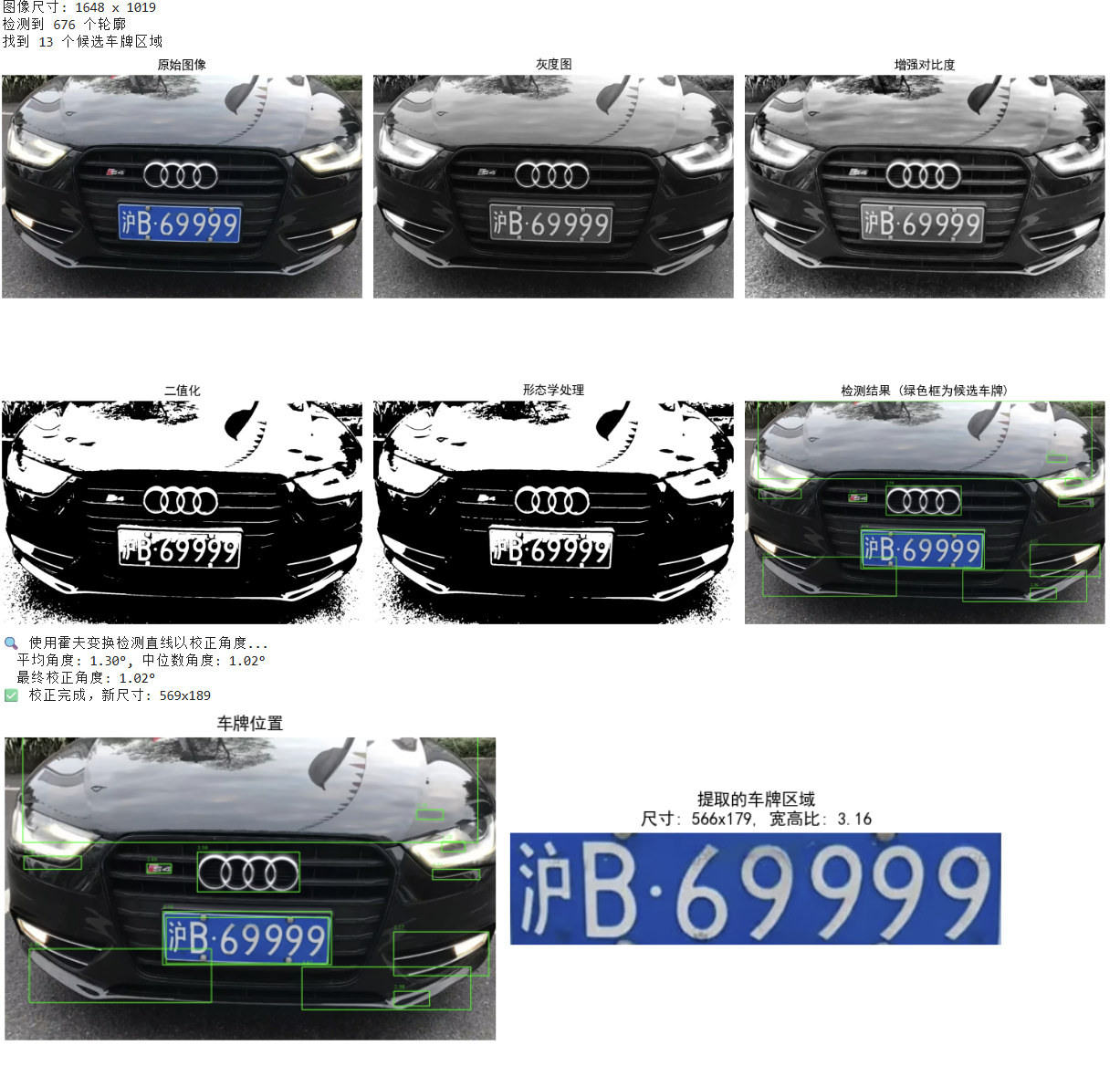
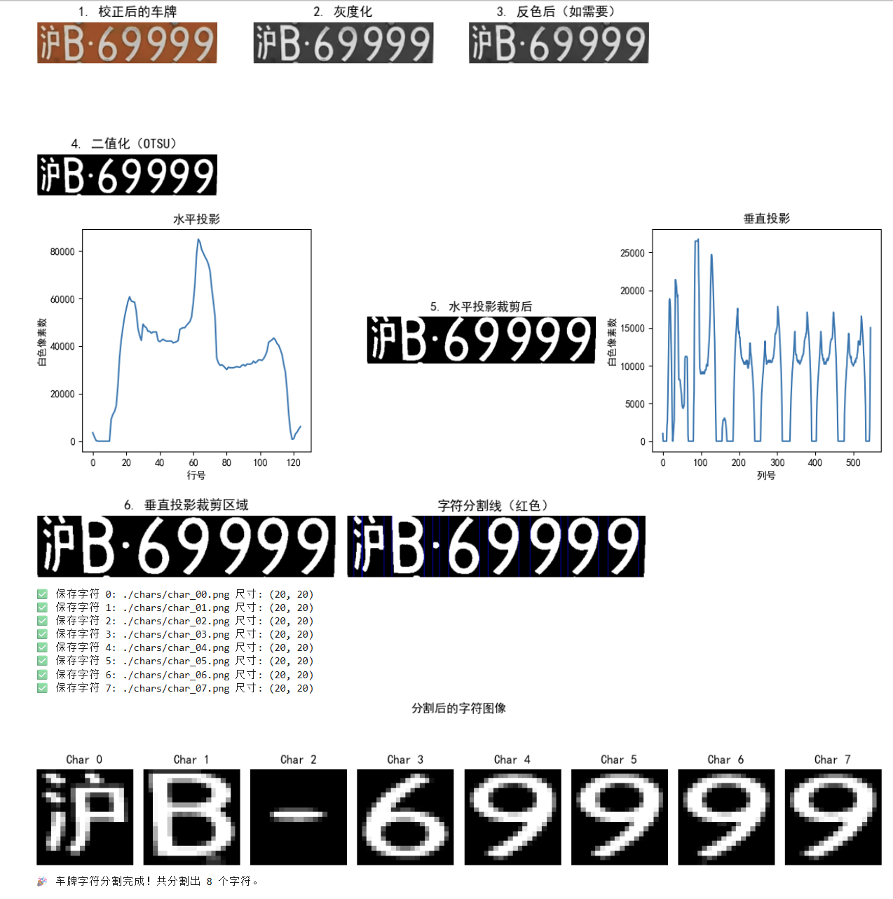
2. 车牌字符分割
前言
定义
提取了车牌,接下来要车牌字符分割
流程:
车牌灰度化--> 黄绿车牌反向-->车牌二值化-->获得车牌区域的水平直方图-->用水平投影去除上下边界-->车牌区域的垂直直方图-->用垂直投影去除左右边界-->组合分离的汉字-->根据字符边界分割字符图像-->给字符图片增加边界,调整图像大小-->保存字符图片
import cv2
import numpy as np
import matplotlib.pyplot as plt
import os
# 设置中文字体支持(可选,用于显示中文标题)
plt.rcParams['font.sans-serif'] = ['SimHei'] # 用来正常显示中文标签
plt.rcParams['axes.unicode_minus'] = False # 用来正常显示负号
# 创建输出目录
os.makedirs('./chars', exist_ok=True)
# ========================
# 读取已校正的车牌图像(假设为彩色)
# ========================
# 替换为你校正后保存的车牌图像路径
plate_img = cv2.imread('./img/corrected_license_plate.jpg')
if plate_img is None:
raise FileNotFoundError("未找到校正后的车牌图像,请检查路径!")
# 转换为 RGB 用于显示
plate_rgb = cv2.cvtColor(plate_img, cv2.COLOR_BGR2RGB)
plate_gray = cv2.cvtColor(plate_rgb, cv2.COLOR_BGR2GRAY)
# 显示原车牌
plt.figure(figsize=(10, 4))
plt.subplot(2, 3, 1)
plt.imshow(plate_rgb)
plt.title('1. 校正后的车牌')
plt.axis('off')
# ========================
# 1. 车牌灰度化(已完成)
# ========================
gray = plate_gray
plt.subplot(2, 3, 2)
plt.imshow(gray, cmap='gray')
plt.title('2. 灰度化')
plt.axis('off')
# ========================
# 2. 黄牌/绿牌反向(如果是深色字浅色底,需反色)
# ========================
# 判断方法:计算平均灰度,若背景亮、字暗 → 反色
mean_val = np.mean(gray)
print(mean_val)
if mean_val > 127: # 假设背景亮(如黄牌、白牌)
gray = 255 - gray # 反色:黑字白底 → 白字黑底(便于二值化)
print("🔄 检测到浅色背景,已进行反色处理")
plt.subplot(2, 3, 3)
plt.imshow(gray, cmap='gray')
plt.title('3. 反色后(如需要)')
plt.axis('off')
# ========================
# 3. 车牌二值化
# ========================
_, binary = cv2.threshold(gray, 0, 255, cv2.THRESH_BINARY + cv2.THRESH_OTSU)
# 使用 OTSU 自动确定最佳阈值,适应不同光照
plt.subplot(2, 3, 4)
plt.imshow(binary, cmap='gray')
plt.title('4. 二值化(OTSU)')
plt.axis('off')
# ========================
# 4. 水平投影:去除上下边框
# ========================
# 计算每一行的白色像素和(投影)
horizontal_projection = np.sum(binary, axis=1) # 沿列方向求和 → 每行总亮度
# 可视化水平投影
plt.figure(figsize=(12, 4))
plt.subplot(1, 3, 1)
plt.plot(horizontal_projection)
plt.title('水平投影')
plt.xlabel('行号')
plt.ylabel('白色像素数')
# 找到上下边界:连续若干行为0的区域
def find_boundaries(projection, min_width=5):
"""找到投影中非零区域的起止索引"""
boundaries = []
start = None
for i, val in enumerate(projection):
if val > 0 and start is None:
start = i
elif val == 0 and start is not None:
if i - start >= min_width: # 忽略过窄区域
boundaries.append((start, i))
start = None
if start is not None and len(projection) - start >= min_width:
boundaries.append((start, len(projection)))
return boundaries
rows = find_boundaries(horizontal_projection, min_width=5)
if rows:
print(rows)
top, bottom = rows[0] # 取第一个连通区域(车牌主体)
# 可适当向内收缩一点,避免边缘噪声
top = max(0, top + 1)
bottom = min(binary.shape[0], bottom - 1)
binary_cropped_h = binary[top:bottom,:]
else:
binary_cropped_h = binary # 未找到则保留原图
top, bottom = 0, binary.shape[0]
plt.subplot(1, 3, 2)
plt.imshow(binary_cropped_h, cmap='gray')
plt.title('5. 水平投影裁剪后')
plt.axis('off')
# ========================
# 5. 垂直投影:去除左右边框并分割字符
# ========================
vertical_projection = np.sum(binary_cropped_h, axis=0) # 每列的白色像素数
plt.subplot(1, 3, 3)
plt.plot(vertical_projection)
plt.title('垂直投影')
plt.xlabel('列号')
plt.ylabel('白色像素数')
plt.tight_layout()
plt.show()
# 找到垂直方向的字符区域
cols = find_boundaries(vertical_projection, min_width=5) # 字符宽度至少3像素
# 过滤掉太窄的区域(可能是噪声)
min_char_width = 1 # 最小字符宽度(像素)
char_regions = [(max(0, left), min(binary_cropped_h.shape[1], right))
for left, right in cols if right - left > min_char_width]
# 显示带分割线的车牌
img_with_lines = cv2.cvtColor(binary_cropped_h, cv2.COLOR_GRAY2BGR)
for left, right in char_regions:
cv2.line(img_with_lines, (left, 0), (left, img_with_lines.shape[0]), (0, 0, 255), 1)
cv2.line(img_with_lines, (right, 0), (right, img_with_lines.shape[0]), (0, 0, 255), 1)
plt.figure(figsize=(8, 3))
plt.subplot(1, 2, 1)
plt.imshow(binary_cropped_h, cmap='gray')
plt.title('6. 垂直投影裁剪区域')
plt.axis('off')
plt.subplot(1, 2, 2)
plt.imshow(img_with_lines)
plt.title('字符分割线(红色)')
plt.axis('off')
plt.tight_layout()
plt.show()
# ========================
# 6. 组合分离的汉字(如“川”、“京”等左右结构)
# ========================
# 简单策略:若两个区域距离很近,且位于前2个字符位置,则合并(适用于中文车牌)
merged_regions = []
i = 0
while i < len(char_regions):
left1, right1 = char_regions[i]
if i + 1 < len(char_regions):
left2, right2 = char_regions[i+1]
gap = left2 - right1
# 如果间距很小(<10像素),且是前两个字符(汉字通常占两个位置)
if gap < 10 and i < 2:
merged_regions.append((left1, right2))
i += 2
continue
merged_regions.append((left1, right1))
i += 1
char_regions = merged_regions if merged_regions else char_regions
# ========================
# 7. 根据字符边界分割字符图像
# ========================
char_images = []
for idx, (left, right) in enumerate(char_regions):
# 提取单个字符
char_img = binary_cropped_h[:, left:right]
# 8. 增加边界(padding),避免字符贴边
char_img_padded = cv2.copyMakeBorder(char_img, 5, 5, 5, 5, cv2.BORDER_CONSTANT, value=0)
# 9. 调整图像大小(统一为 20x20 或 32x32,便于OCR)
char_img_resized = cv2.resize(char_img_padded, (20, 20), interpolation=cv2.INTER_AREA)
# 保存字符图像
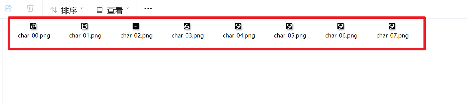
char_filename = f'./chars/char_{idx:02d}.png'
cv2.imwrite(char_filename, char_img_resized)
char_images.append(char_img_resized)
print(f"✅ 保存字符 {idx}: {char_filename} 尺寸: {char_img_resized.shape}")
# ========================
# 10. 显示所有分割后的字符
# ========================
plt.figure(figsize=(12, 3))
for i, char_img in enumerate(char_images):
plt.subplot(1, len(char_images), i+1)
plt.imshow(char_img, cmap='gray')
plt.title(f'Char {i}')
plt.axis('off')
plt.suptitle('分割后的字符图像')
plt.tight_layout()
plt.show()
print("🎉 车牌字符分割完成!共分割出", len(char_images), "个字符。")